2.1.3.2 Probability of an event

We denote the joint Probability of events A and B both happening as follows:

If A and B are independent events, we have:

2.1.3.3 Probability of a union of two events

The probability of evetnt A or B happening is given by:

If the events are mutually exclusive (so they cannot happen at the same time), we get:

2.1.3.4 Conditional probability of one event given another

We define the conditional probability of event B happening given that A has occurred as follows:

2.1.3.5 Independence of events

We say that event A is independent of event B if:

2.1.3.6 Conditional independence of events

We say taht events A and B are conditionally independent given event C if:

This is written as $A \bot B|C$. Events are often dependent on each other, but may be rendered independent if we condition on the relevant intermediate variables.

2.2 Random variables

If the value of $X$ is unknown and/or cound change, we call it a random variable or rv. The set of possible values, denoted $\mathcal{X}$, known as the sample space or state space.

2.2.1 Discrete random variables (pmf)

If the sample space $\mathcal{X}$ is finite or countably infinite, then $X$ is called a discrete random variable. In this case, we denote the probability of the event that $X$ has value $x$ by $Pr(X=x)$. We define the probability mass function or pmf as a function which computes the probability of events which correspond to setting the rv to each possible value:

$0 \leq p(x) \leq 1$ and $\sum_{x \in \mathcal{X}} p(x)=1$

2.2.2 Continuous random variables

If $X \in \mathbb{R}$ is a real-valued quantity, it is called a continuous random variable.

2.2.2.1 Cumulative distribution function (cdf)

Define the events $A=(X \leq a)$, $B=(X \leq b)$ and $C=(a < X \leq b)$, where $a<b$. We have that $B=A \vee C$, and since $A$ and $C$ are mutually exclusive, the sum rules gives:

and hence the probability of being in interval $C$ is given by

In general, we define the cumulative distribution function or cdf of the $rv$ $X$ as follows:

Using this, we can compute the probability of being in any interval as follows:

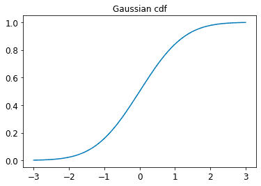
Here is an example of cdf for standard normal distribution: $\mathcal N (x|0,1)$

2.2.2.2 probability density function (pdf)

We define the probability density function or pdf as the derivative of the cdf:

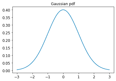
Example of pdf for standard normal distribution: $\mathcal N (x|0,1)$

Given a pdf, we can compute the probability of a continuous variable being in a finite interval as follows:

As the size of the interval gets smaller, we can write

2.2.2.3 Quantiles (percent point function, ppf)

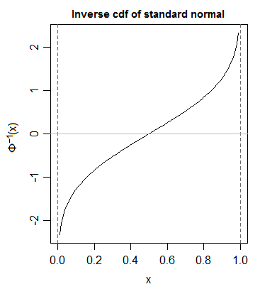
If the cdf $P$ is strictly monotonically increasing, it has an inverse, called the inverse cdf, or percent point function (ppf), or quantile function. For example, let $\Phi$ be the cdf of Gaussian distribution $\mathcal N (x|0,1)$, and $\Phi^{-1}$ be the inverse cdf.

If the distribution is $\mathcal N (\mu, \sigma^2)$, then 95% interval becomes ($\mu-1.96\sigma, \mu+1.96\sigma$). This is often approximated by writing $\mu \pm 2\sigma$

2.2.3 Sets of related random variables

We have two random variables, $X$ and $Y$. We can define the joint distribution of two random variables using $p(x, y)=p(X=x, Y=y)$ for all possible values of $X$ and $Y$. With finite cardinality, we can represent the joint distribution as a 2d table:

Given a joint distribution, we define the marginal distribution of an rv as follows:

This is also called the sum rule.

We difine the conditional distribution of an rv using

We can rearrange this equation to get

This is called the product rule.

By extending the product rule to $D$ variables, we get the chain rule of probability:

2.2.4 Independence and conditional independence

We say $X$ and $Y$ are unconditional independent or marginally independent, denoted $X \bot Y$, if we can represent the joint as the product of the two marginals, i.e.,

In general, we say a set of variables $X_1, ... , X_n$ is independent if the joint can be written as a product of marginals, i.e.,

Unconditional independence is rare. We therefore say $X$ and $Y$ are conditionally independent (CI) given $Z$ iff the conditional joint can be written as a product of conditional marginals:

2.2.5 Mean of a distribution

For continuous rv's, the mean is defined as follows:

For discrete rv's, mean:

Mean is a linear operator, we have

This is called linearty of expectation.

For a set of $n$ rv's, one can show that the expectation of their sum is as follows:

If they are independent, the expectation of their product is given by

2.2.5.2 Variance of a distribution

The variance is a measure of the "spread" of a distribution, often denoted by $\sigma^2$.

from which we derive the useful result:

The standard deviation is defined as:

This is useful since it has the same units as $X$ itself.

Shifted and scaled variance:

Variance of the sum of a set of $n$ independent random variables: $\mathbb[\sum^n_{i=1}X_i]=\sum^n_{i=1}\mathbb{V}[X_i]$

Variance of the product of a set of $n$ independent random variables: $\mathbb{V}[\prod^n_{i=1}X_i]=\prod_i(\sigma^2_i+\mu^2_i)-\prod_i\mu^2_i$

2.2.5.3 Mode of a distribution

The mode of a distribution is the value with the highest probability mass or probability density:

2.2.5.4 Conditional moments

When we have two or more dependent random variables, we can compute the moments of one given knowledge of the other. For example, the law of iterated expectations, also called the law of total expetation, tells us that:

Similarly, for variance, we have the law of total variance, also called the conditional variance formula, tells us that:

2.3 Bayes' rule